circle
circular functions
coefficient
combination
| A | B | C | D | E | F | G | H | I | JKL | MN | O | P | Q | R | S | T | UV | WXYZ |
|---|---|---|---|---|---|---|---|---|---|---|---|---|---|---|---|---|---|---|
| Algebra 2 Connections Glossary | ||||||||||||||||||
circle |
|
|---|---|
| In a plane, the set of all points equidistant from a single point. The general equation of a circle is (x − h)2 + (y − k)2 = r2 where the point (h, k) is the center of the circle of radius r. (pp. 198, 206, 566, 567, 576) | |
circular functions |
|
| The periodic functions based on the unit circle, including y = sin x, y = cos x, and y = tan x . See “sine function,” “cosine function,” and “tangent function.” | |
coefficient |
|
| When variable(s) are multiplied by a number, the number is called a coefficient of that term. The numbers that are multiplied by the variables in the terms of a polynomial are called the coefficients of the polynomial. For example, 3 is the coefficient of 3x2. (p. 440) | |
combination |
|
| A combination is the number of ways we can select items from a larger set without regard to order. For instance, choosing a committee of 3 students from a group of 5 volunteers is a combination since the order in which committee members are selected does not matter. We write nCr to represent the number of combinations of n things taken r at a time (or n choose r). For instance, the number of ways to select a committee of 3 students from a group of 5 is 5C3. You can use Pascal’s Triangle to find 5C3or use permutations and divided by the number of arrangements | |
common difference |
|
|---|---|
| The difference between consecutive terms of an arithmetic sequence or the generator of the sequence. When the common difference is positive the sequence increases; when it is negative the sequence decreases. In the sequence 3, 7, 11, ..., 43, the common difference is 4. (pp. 75, 83) | |
common ratio |
|
| Common ratio is another name for the multiplier or generator of a geometric sequence. It is the number to multiply one term by to get the next one. In the sequence: 96, 48, 24, … the common ratio is
|
|
complete graph |
|
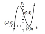
| A complete graph is one that includes everything that is important about the graph (such as intercepts and other key points, asymptotes, or limitations on the domain or range), and that makes the rest of the graph predictable based on what is shown. For example, a complete graph of the equation |
|
completing the square |
|
| A standard procedure for rewriting a quadratic equation from standard form to graphing (or vertex) form is called completing the square. Completing the square is also used to solve quadratic equations in one variable. For example, the expression x2 − 6x + 4 starts with the first two terms of (x − 3)2. To “complete the square” we need to add 9 to x2 − 6x. Since the original expression only adds 4, completing the square would increase the expression by 5, so (x − 3)2 − 5 is an equivalent form that is useful for solving or graphing. (pp. 202, 206, 387) | |
complex conjugates |
|
| The complex number a + bi has a complex conjugate a − bi. Similarly, the conjugate of c − di is c + di . What is noteworthy about complex numbers conjugates is that both their product (a + bi)(a − bi) = a2 − b2i2 = a2 + b2 and their sum (a + bi) + (a − bi) = 2a are real numbers. If a complex number is a zero (or root) of a real polynomial function, then its complex conjugate is also a zero (or root). (p. 460) | |
complex numbers |
|
Numbers written in the form a + bi where a and b are real numbers, are called complex numbers. Each complex number has a real part, a, and an imaginary part, bi. Note that real numbers are also complex numbers with b = 0 , and imaginary numbers are complex numbers where a = 0. (pp. 455, 456)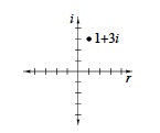 |
|
complex plane |
|
| A set of coordinate axes with all the real numbers on the horizontal axis (the real axis) and all the imaginary numbers on the vertical axis (the imaginary axis) defines the complex plane. Complex numbers are graphed in the complex plane using the same method we use to graph coordinate points. Thus, the complex number 1 + 3i is located at the point (1, 3) in the complex plane. (p. 466) | |
composite function |
|
| A function that is created as the result of using the outputs of one function as the inputs of another can be seen as a composite function. For example the function h(x) = |log x| can be seen as the composite function f(g(x)) where f(x) = |x| and g(x) = log x . See “composition.” (p. 292) | |
composition |
|
| When the output of one function is used as the input for a second function, a new function is created which is a composition of the two original functions. If the first function is g(x) and the second is f(x), the composition can be written as f(g(x)) or f 0g(x) . Note that the order in which we perform the functions matters and g(f(x)) will usually be a different function. (p. 274) | |
compound interest |
|
|---|---|
| Interest that is paid on both the principal and the previously accrued interest. (pp. 125, 658, 661) | |
compress |
|
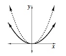
| A term used informally to describe the relationship of a graph to its parent graph when the graph increases or decreases more slowly than the parent. For example, the solid parabola shown below is a compressed version of its parent, shown as a dashed curve. (pp. 170, 175)
|
|
conditional probability |
|
| The probability of outcome B occurring, given that outcome A has already happened is called the conditional probability of B, given A (the usual notation is P(B|A) ). One way to calculate the conditional probability of B given A, is to divide the probability of both outcomes A and B by the probability of outcome A alone, or |
|
cone |
|
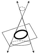
| If you have a circle in a plane and a point P, not in that plane, the solid obtained by joining all of the points inside or on the circle to P is a circular cone. P is called the apex of the cone. A standard cone is a circular cone with its apex P directly over the center of the circle. For the purpose of defining the conic sections visualize two standard cones, one upside down on top of the other, touching at their apexes and both extending infinitely, one upwards and one downwards. (p. 554)
|
|
conic section |
|
| Circles, ellipses, hyperbolas and parabolas are known as conic sections. They are given this name because each curve can be found by taking a section or slice of a cone. (pp. 554, 561) | |
conjugate |
|
| Every complex number a + bi has a conjugate, a − bi , and both the sum and product of the conjugates are real. Similarly, an irrational number that can be written |
|
conjugate axis |
|
| The axis of a hyperbola that does not contain the vertices. It is perpendicular to the transverse axis at the center of the hyperbola. The distance from the center to the end of the conjugate axis is represented as b in the general equation. (p. 585) See “hyperbola.” | |
continuous |
|
| For this course, when the points on a graph are connected and it makes sense to connect them, we say the graph is continuous. Such a graph will have no holes or breaks in it. This term will be more completely defined in a later course. (pp. 62, 86) | |
coordinate axes |
|
| For two dimensions, two perpendicular number lines, the x‑ and y‑axes, that intersect where both are zero and that provide the scale(s) for labeling each point in a plane with its horizontal and vertical distance and direction from the origin (0, 0). In three dimensions, a third number line, the z‑axis, is perpendicular to a plane and intersects it at origin (0, 0, 0). The z‑axis provides the scale for the height of a point above or below the plane. See“3‑dimensional coordinate system.” (p. 307)
|
|
coordinates |
|
|---|---|
| The numbers in an ordered pair (a, b) or triple (a, b, c) used to locate a point in the plane or in space in relation to a set of coordinate axes. (pp. 22, 307)
|
|
cosecant |
|
| The cosecant is the reciprocal of the sine. (p. 682) | |
cosine |
|
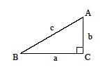
| In a right triangle (as shown below the ratio
|
|
cosine function |
|
The cosine of angle θ, denote cos θ , is the x‑coordinate of the point on the unit circle reached by a rotation angle of θ radians in standard position. The general equation for the cosine function is y = acos b(x − h) + k. This function has amplitude a, period 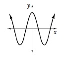 |
|
cosine inverse (cos−1x) |
|
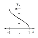
| Read as the inverse of cosine x, cos−1x is the measure of the angle with cosine x. We can also write y = arc cos x . Note that the notation refers to the inverse of the cosine function, not
|
|
cotangent |
|
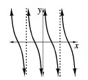
| The cotangent is the reciprocal of the tangent. The graph of the cotangent function is below. (p. 683)
|
|
cubic |
|
| A cubic polynomial is a polynomial with degree 3. (pp. 182, 207) | |
cycle |
|
| One cycle of a graph of a trigonometric function is the shortest piece that represents all possible outputs. The length of one cycle is the distance along the x‑axis needed to generate all possible output values or the distance around the unit circle needed to generate all possible outcomes. (p. 379)
|
|
cyclic function |
|
| The term cyclic function is sometimes used to describe trigonometric functions, but it also includes any function that sequentially repeats its outputs at regular intervals. (p. 412) | |